Using Tensorflow and Support Vector Machine to Create an Image Classifications Engine

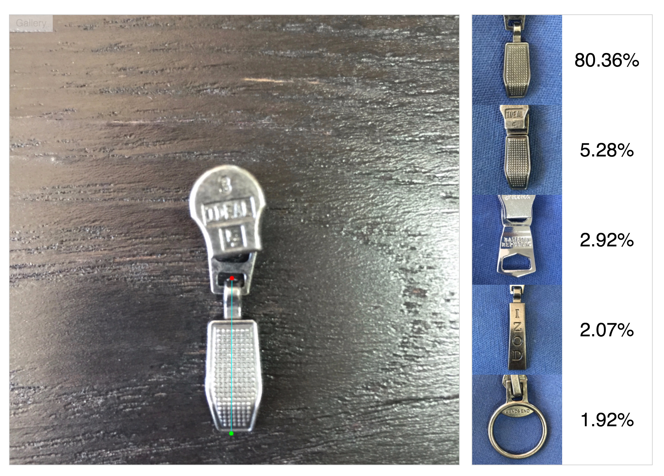
In this post, we are documenting how we used Google’s TensorFlow to build this image recognition engine. We’ve used Inception to process the images and then train an SVM classifier to recognise the object. Our aim is to build a system that helps a user with a zip puller to find a matching puller in the database. This piece will also cover how the Inception network sees the input images and assess how well the extracted features can be classified.

Our puller project with Tensorflow

Recently, Oursky got a mini zip puller recognition project. One of our teams had to build a system for users to match an image of puller with most similar puller inside the database. The sample size for the trial is small (12 pullers), which has implications discussed below as we share our experience on trying out Google’s TensorFlow.

Our first test was to compare the HoG (Histogram of Oriented Gradient) feature computed on the input image and all the puller model images rendered from their CAD models. This solution works but the matching performance is poor if the input image background has a strong texture.

We also tested an alternative solution to address the problems with the textured background. We then built a relatively shallow CNN with 2 convolutional layers and two fully connected layer ¹ for classifying the puller image. However, since our data set is too small (around 200 puller images for each type) and lacks variety, the classification performance is poor. It is basically not different from making random guesses.

Training a CNN from scratch with a small data set is indeed a bad idea. The common approach for using CNN to do classification on a small data set is not to train your own network, but to use a pre-trained network to extract features from the input image and train a classifier based on those features. This technique is called transfer learning. TensorFlow has a tutorial on how to do transfer learning on the Inception model; Kernix also has a nice blog post talking about transfer learning and our work is largely based on that.

Brief overview on classification

In a classification task, we first need to gather a set of training examples. Each training example is a pair of input features and labels. We would like to use these training examples to train a classifier, and hope that the trained classifier can tell us a correct label when we feed it an unseen input feature.

There are lots of learning algorithms for classification, e.g. support vector machine, random forest, neural network, etc. How well a learning algorithm can perform is highly related to the input feature. Input feature is a representation that captures the essence of the object under classification.

For example, in image recognition, the raw pixel values could be an input feature. However, using raw pixel values as input feature, the feature dimension is usually too big or too generic for a classifier to work well. In this case, we can either use a more complex classifier such as deep neural network, or use some domain knowledge to brainstorm a better input feature.²

For our puller classification task, we will use SVM for classification, and use a pre-trained deep CNN from TensorFlow called Inception to extract a 2048-d feature from each input image.

Bottlenecks features of deep CNN

The common structure of a CNN for image classification has two main parts: 1) a long chain of convolutional layers, and 2) a few (or even one) layers of the fully connected neural network. The long convolutional layer chain is indeed for feature learning. The learned feature will be feed into the fully connected layer for classification.

The feature that feeds into the last classification layer is also called the bottleneck feature. The following image shows the structure of TensorFlow’s Inception network we are going to use. We have indicated the part of the network that we are getting the output from as our input feature.

How Inception sees a puller

Training a CNN means it learns a bunch of (https://en.wikipedia.org/wiki/Kernel_(image_processing).

For example, if the input of the convolutional layer is an image with 3 channels, the kernel size for this layer is 3×3 and there will be an independent set of three 3×3 kernels for each output channel. Each kernel in a set will convolve with the corresponding channel of the input and produces three convolved images. The sum of those convolved images will form a channel of the output.

The illustration below is a convolution step.

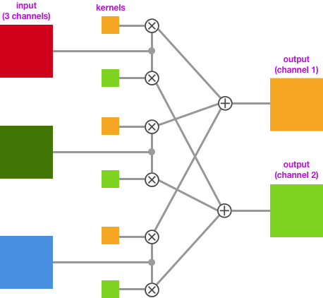
As the output of each convolutional layer ³ is a multi-channel image, we could also view them as multiple gray-scale images.”. By plotting those grayscale images out, we can understand how the Inception network sees an image. The following images are extracted at different stages of the convolutional layer chain The points are illustrated as A,B,C and D in the Inception Model figure.

This is an input image.

All the 32 149×149 images at stage A:

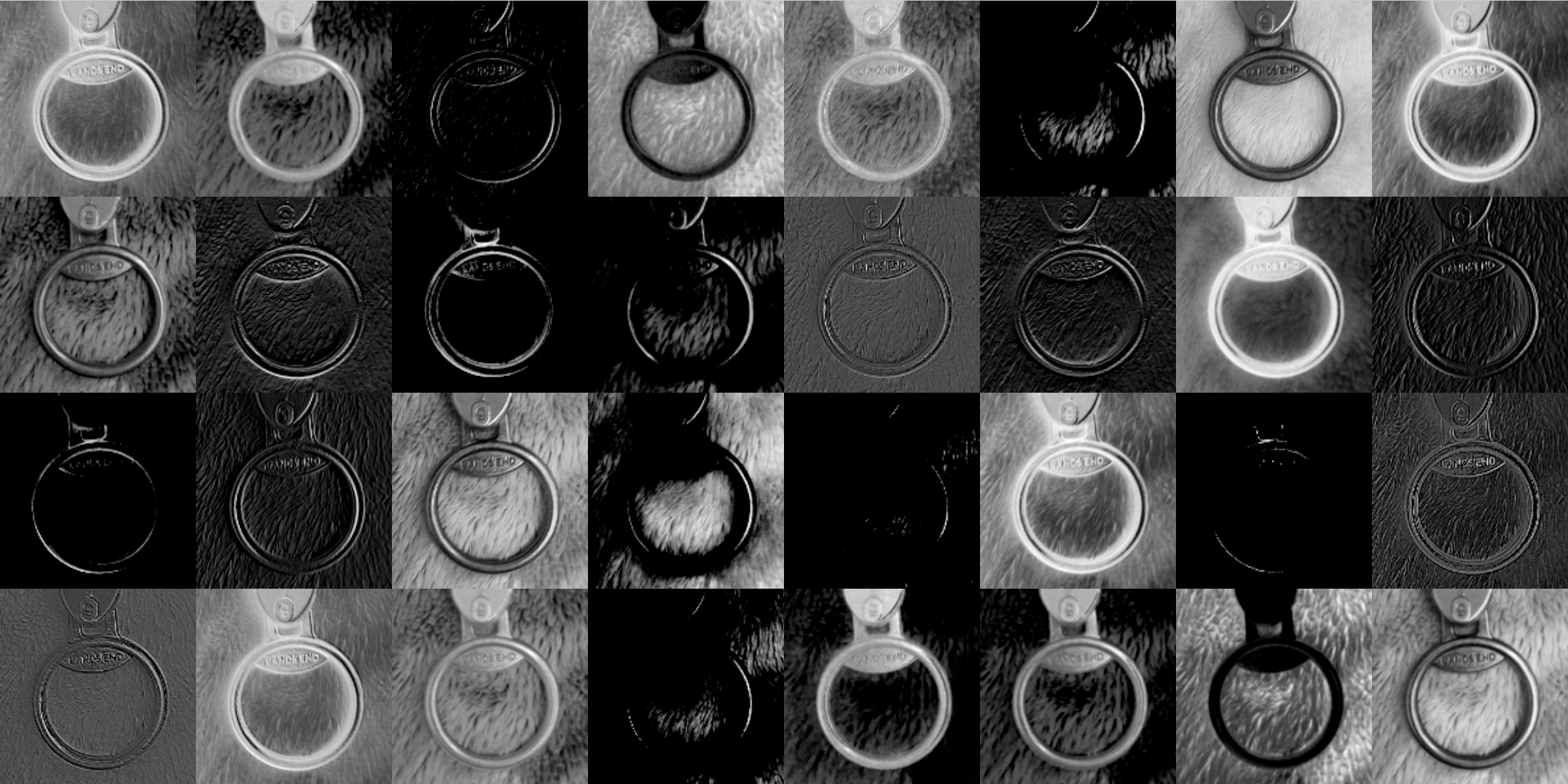
All the 32 147×147 images at stage B:

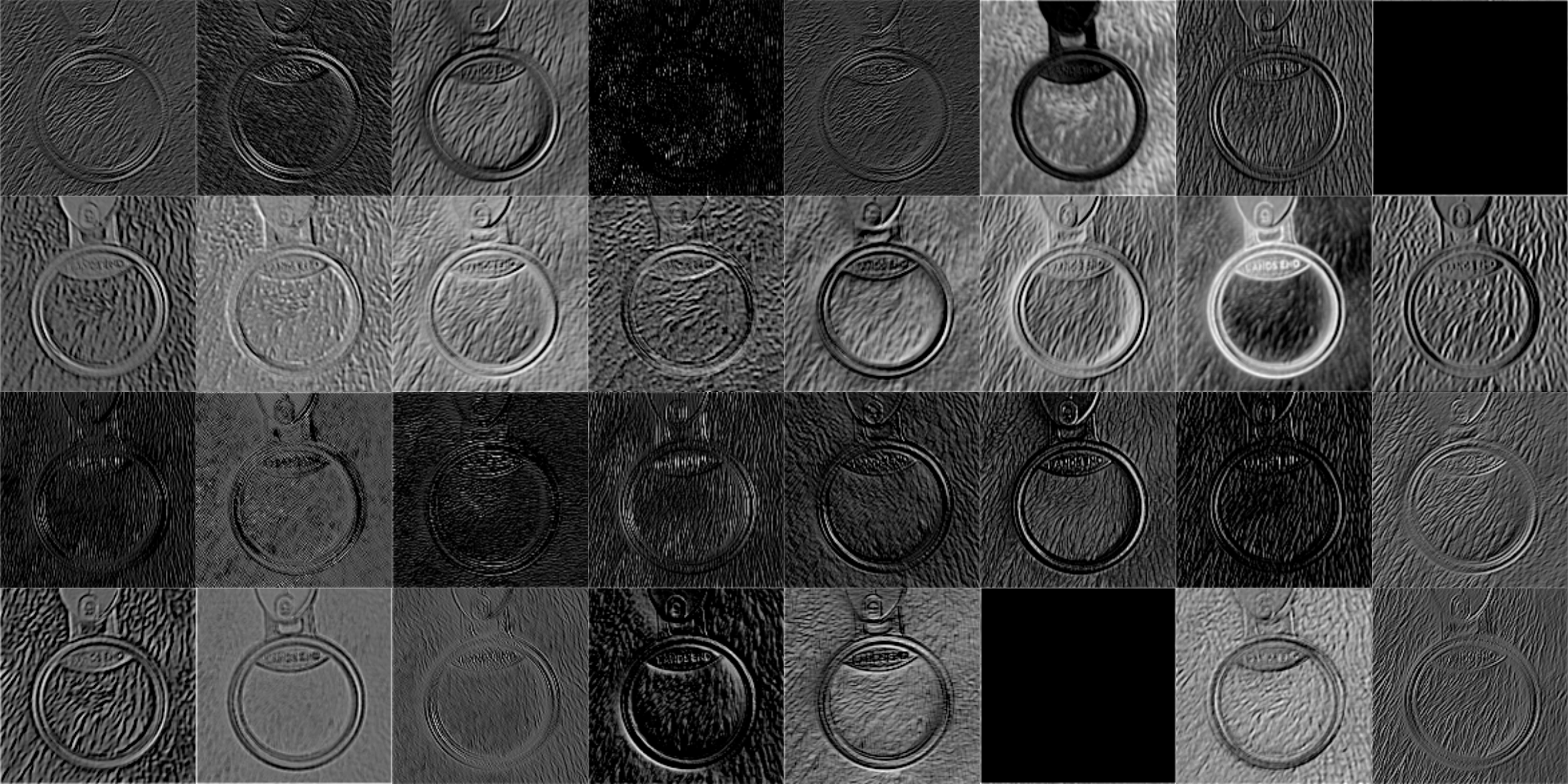
All the 288 35×35 images at stage C:

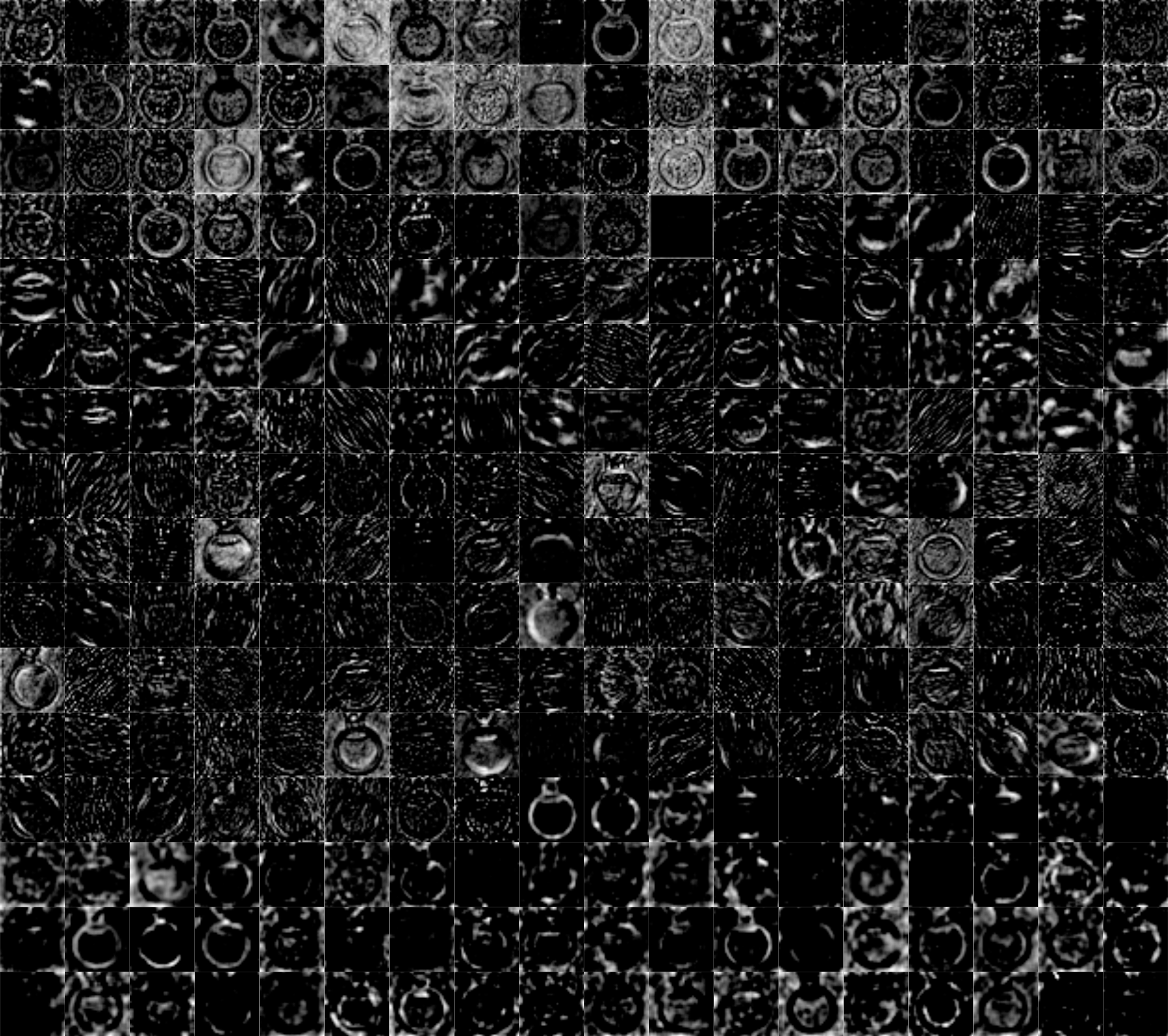
All the 768 17×17 images at stage D:

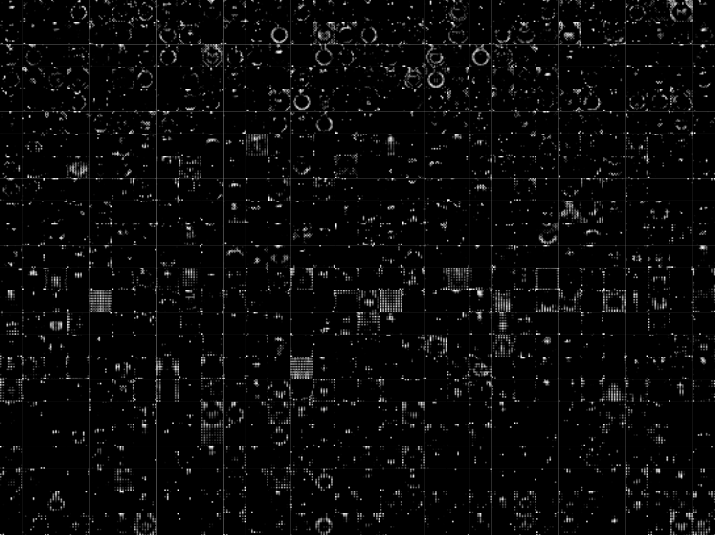
Here we can see the images become more and more abstract going down the convolutional layer chain. We could also spot that some of the image are highlighting the puller, and some of them are highlighting the background.

Why is the bottleneck feature is good?

The bottleneck feature of Inception network is a 2048-d vector. The following is a figure showing the bottleneck feature of the previous input image in bar chart form.

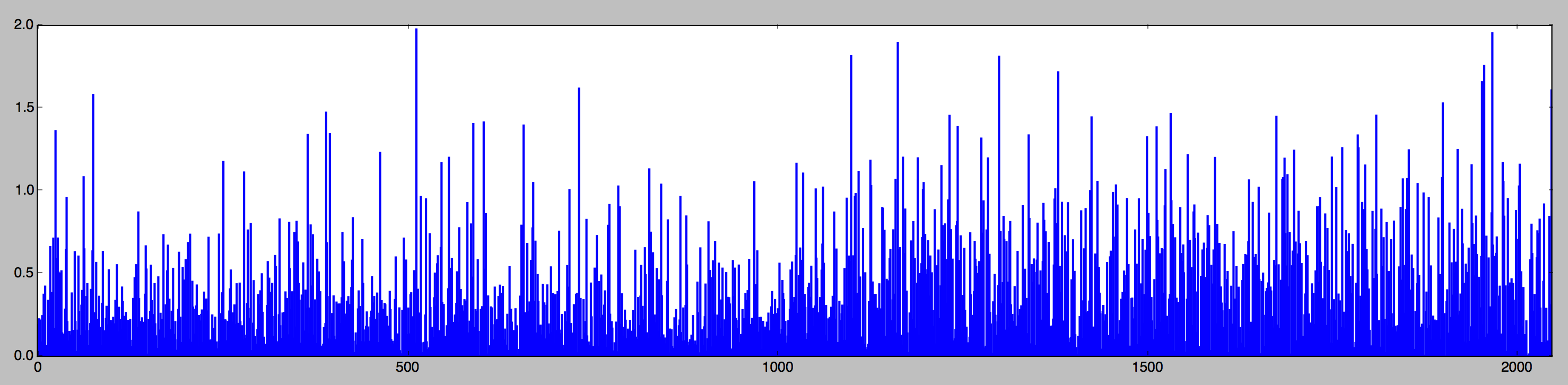
For the bottleneck feature to be a good feature for classification, we would like the features representing the same type of puller to be close (think of the feature as a point in 2048-d space) to each other, while features representing different types of puller should be far apart. In other words, we would like to see features in a data set clustering themselves according to their types.

It is hard to see this kind of clustering happened on 2048-d feature data sets. However, we can do a dimensionality reduction⁴ on the bottleneck feature and transform them to a 2-d feature which is easy to visualize. The following image is the scatter plot of the transformed feature in our puller data set⁵. Different puller type are illustrated by different colors.

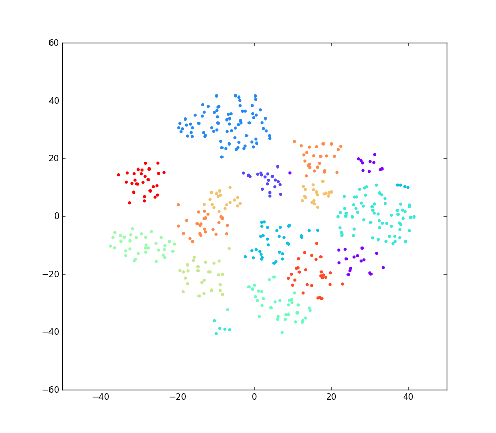
As we can see, the same color points are mostly clustered together. It has a high chance that we could use the bottleneck feature to train a classifier with high accuracy.

Code for extracting inception bottleneck feature

import tensorflow as tf
import tensorflow.python.platform
from tensorflow.python.platform import gfile
import numpy as np

def create_graph(model_path):
    """
    create_graph loads the inception model to memory, should be called before
    calling extract_features.

    model_path: path to inception model in protobuf form.
    """
    with gfile.FastGFile(model_path, 'rb') as f:
        graph_def = tf.GraphDef()
        graph_def.ParseFromString(f.read())
        _ = tf.import_graph_def(graph_def, name='')


def extract_features(image_paotths, verbose=False):
    """
    extract_features computed the inception bottleneck feature for a list of images

    image_paths: array of image path
    return: 2-d array in the shape of (len(image_paths), 2048)
    """
    feature_dimension = 2048
    features = np.empty((len(image_paths), feature_dimension))

    with tf.Session() as sess:
        flattened_tensor = sess.graph.get_tensor_by_name('pool_3:0')

        for i, image_path in enumerate(image_paths):
            if verbose:
                print('Processing %s...' % (image_path))

            if not gfile.Exists(image_path):
                tf.logging.fatal('File does not exist %s', image)

            image_data = gfile.FastGFile(image_path, 'rb').read()
            feature = sess.run(flattened_tensor, {
                'DecodeJpeg/contents:0': image_data
            })
            features = np.squeeze(feature)

    return features 

The inception v3 model can be downloaded here.

Training a SVM classifier

Support vector machine (SVM) is a linear binary classifier.

The goal of the SVM is to find a hyper-plane that separates the training data correctly in two half-spaces while maximising the margin between those two classes.

Although SVM is a linear classifier, which could only deal with linear separable data sets, we can apply a kernel trick to make it work for non-linear separable case.

A commonly used kernel besides linear is the RBF kernel.

The hyper-parameters for SVM includes the type of kernel and the regularization parameter C. If using the RBF kernel, there is an additional parameter γ for selecting which radial basic function to use.

Usually the bottleneck feature from a deep CNN is linear separable. However, we will consider the RBF kernel as well.

We used simple grid search for selecting the hyper-parameter. In other words, we tried out all the hyper-parameter combination in the range we have specified, and evaluated the trained classifier performance using cross validation.

The rule of thumb for trying out the C and γ parameter is trying them with different order of magnitude.

We used 10-fold cross validation.

SVM is a binary classifier. However, we could use the one-vs-all or one-vs-one approach to make it a multi-class classifier.

It seems a lot of stuff to do for training a SVM classifier, indeed it is just a few function calls when using machine learning software package like scikit-learn.

Code for the training the SVM classifier

import os

import sklearn
from sklearn import cross_validation, grid_search
from sklearn.metrics import confusion_matrix, classification_report
from sklearn.svm import SVC
from sklearn.externals import joblib

def train_svm_classifer(features, labels, model_output_path):
    """
    train_svm_classifer will train a SVM, saved the trained and SVM model and
    report the classification performance

    features: array of input features
    labels: array of labels associated with the input features
    model_output_path: path for storing the trained svm model
    """
    # save 20% of data for performance evaluation
    X_train, X_test, y_train, y_test = cross_validation.train_test_split(features, labels, test_size=0.2)

    param = [
        {
            "kernel": ["linear"],
            "C": [1, 10, 100, 1000]
        },
        {
            "kernel": ["rbf"],
            "C": [1, 10, 100, 1000],
            "gamma": [1e-2, 1e-3, 1e-4, 1e-5]
        }
    ]

    # request probability estimation
    svm = SVC(probability=True)

    # 10-fold cross validation, use 4 thread as each fold and each parameter set can be train in parallel
    clf = grid_search.GridSearchCV(svm, param,
            cv=10, n_jobs=4, verbose=3)

    clf.fit(X_train, y_train)

    if os.path.exists(model_output_path):
        joblib.dump(clf.best_estimator_, model_output_path)
    else:
        print("Cannot save trained svm model to {0}.".format(model_output_path))

    print("\nBest parameters set:")
    print(clf.best_params_)

    y_predict=clf.predict(X_test)

    labels=sorted(list(set(labels)))
    print("\nConfusion matrix:")
    print("Labels: {0}\n".format(",".join(labels)))
    print(confusion_matrix(y_test, y_predict, labels=labels))

    print("\nClassification report:")
    print(classification_report(y_test, y_predict))

SVM training result

The following is the training result we get, which got a perfect result! Though this might deal to overfitting…

Best parameters set:
{'kernel': 'linear', 'C': 1}

Confusion matrix:
Labels: 8531,8539,8567,8568,8599,8715,8760,8773,8777,8778,8808,8816

[[ 4  0  0  0  0  0  0  0  0  0  0  0]
 [ 0  2  0  0  0  0  0  0  0  0  0  0]
 [ 0  0 12  0  0  0  0  0  0  0  0  0]
 [ 0  0  0  9  0  0  0  0  0  0  0  0]
 [ 0  0  0  0 19  0  0  0  0  0  0  0]
 [ 0  0  0  0  0  8  0  0  0  0  0  0]
 [ 0  0  0  0  0  0  8  0  0  0  0  0]
 [ 0  0  0  0  0  0  0  5  0  0  0  0]
 [ 0  0  0  0  0  0  0  0  9  0  0  0]
 [ 0  0  0  0  0  0  0  0  0 11  0  0]
 [ 0  0  0  0  0  0  0  0  0  0  5  0]
 [ 0  0  0  0  0  0  0  0  0  0  0  4]]

Classification report:
             precision    recall  f1-score   support

       8531       1.00      1.00      1.00         4
       8539       1.00      1.00      1.00         2
       8567       1.00      1.00      1.00        12
       8568       1.00      1.00      1.00         9
       8599       1.00      1.00      1.00        19
       8715       1.00      1.00      1.00         8
       8760       1.00      1.00      1.00         8
       8773       1.00      1.00      1.00         5
       8777       1.00      1.00      1.00         9
       8778       1.00      1.00      1.00        11
       8808       1.00      1.00      1.00         5
       8816       1.00      1.00      1.00         4

avg / total       1.00      1.00      1.00        96

We’ve used it to built an mobile app and a web front-end for the puller classifier for field testings.

Since the classifier can work with unseen samples, it seems that the over-fitting issue is not so serious.

Conclusion

A pre-trained deep CNN, Inception network in particular, could be used as a feature extractor for general image classification tasks.

The bottleneck feature of the Inception network should a good feature for classification. We have extracted the bottleneck feature from our data set and did a dimensionality reduction for visualization. The result shows a nice clustering of the sample according to their class.

The SVM classifier training on the bottleneck feature has a perfect result, and the classifier seems to work on the unseen sample.

Footnotes